

Survey grids — also called sampling grids or fishnet grids — divide a field into equal-area cells for systematic drone and aerial survey sampling, trial plot layouts, inspection zones, and report maps. Generating one manually in QGIS is straightforward but repetitive. This script does it in one run with automatic CRS handling.
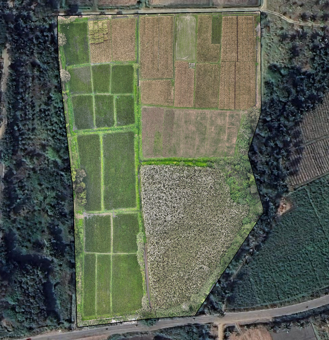
Here’s the field before gridding — just the raw drone orthomosaic with the outer boundary marked:
What it does
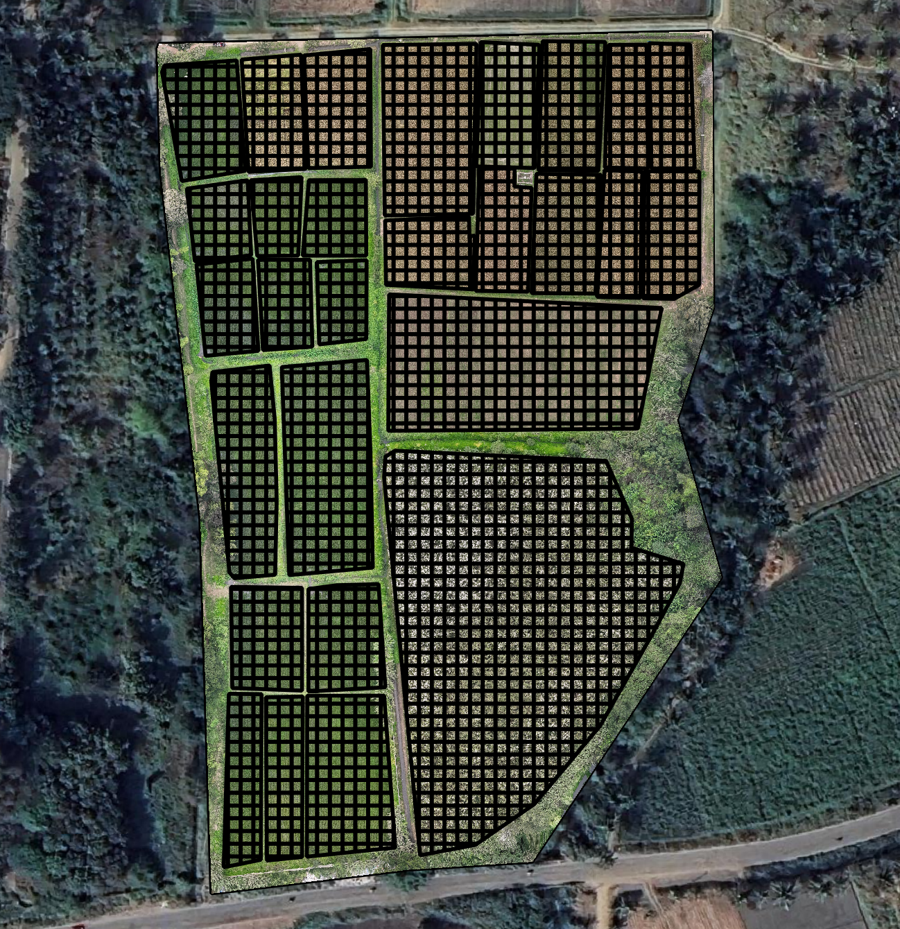
The grid_generation.py script creates a regular rectangular grid of equal-sized cells in metres. If polygon GeoJSON layers are checked (visible), the grid is clipped to their combined shape — only cells that fall inside the polygons are kept. If no polygon layers are visible, the grid covers the current canvas extent.
The script automatically detects geographic CRS (latitude/longitude in degrees) and reprojects to the appropriate UTM zone so the cell size you set is in real metres, not degrees.
Output: grid_clipped.geojson saved in the same directory as the first checked polygon layer, loaded into the QGIS project.
What you need
- QGIS 3.28 or newer
numpy, QGIS processing framework (both bundled with QGIS)- (Optional) polygon GeoJSON layers checked in the Layers panel to clip the grid
- The
grid_generation.pyscript from the Drone Mapping, Terrain & Multispectral Analysis QGIS Package
Steps
-
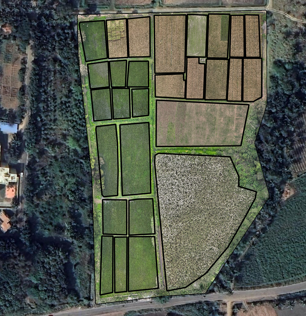
Load your boundary polygon (or multipolygon) layer into QGIS and check (tick) it in the Layers panel — a per-plot field boundary layer like this one works well, since the grid is clipped to the combined shape of every polygon in it:
-
Open Plugins → Python Console → Show Editor.
-
Paste the script. At the bottom, set:
cell_size_m— the width and height of each grid cell in metres (e.g.50for a 50×50 m grid)
-
Click Run.
Checked, not active: the polygon layer only needs to be checked (ticked) in the Layers panel — it does not need to be the active (selected/highlighted) layer, and this script never reads iface.activeLayer(). It also doesn’t need to be checked at all, strictly speaking: this input is optional, not mandatory. If no polygon .geojson layer is checked, the script doesn’t error — it falls back to gridding the current map canvas extent instead. That’s useful for a quick reference grid, but the output won’t be clipped to your field shapes. It still lands in the right place though — the script infers your project folder from the open QGIS project file and saves to its 2.Session/Geojsons/ folder (creating it if it doesn’t already exist — see the recommended project folder structure), same as it would next to a checked polygon layer. For a real per-field grid, make sure your boundary layer is ticked before running.
Configurable parameters
| Parameter | What it controls |
|---|---|
cell_size_m | Width and height of each cell in metres |
Common uses
- Sample plot grids — divide a field into equal-area cells for systematic soil or crop sampling
- Inspection zones — create reference cells for aerial survey coverage planning
- Report maps — overlay a scale grid on a map layout for reference
Why cell size matters: a raw sensor raster — NDVI or otherwise — gives you a value per pixel, often just centimetres across. No sprayer, drone applicator, or field crew can act at that resolution; you can’t treat one 5 cm patch differently from the one next to it. Averaging the raster within each grid cell collapses that pixel-level noise into a single number per cell, turning the raster into a set of decision-making areas you can actually act on — spray this cell, skip that one, flag another for manual inspection. In precision agriculture this is often called a management or prescription zone, and cell_size_m is where you draw the line between “more detail than anyone can act on” and “coarse enough to actually act on.”
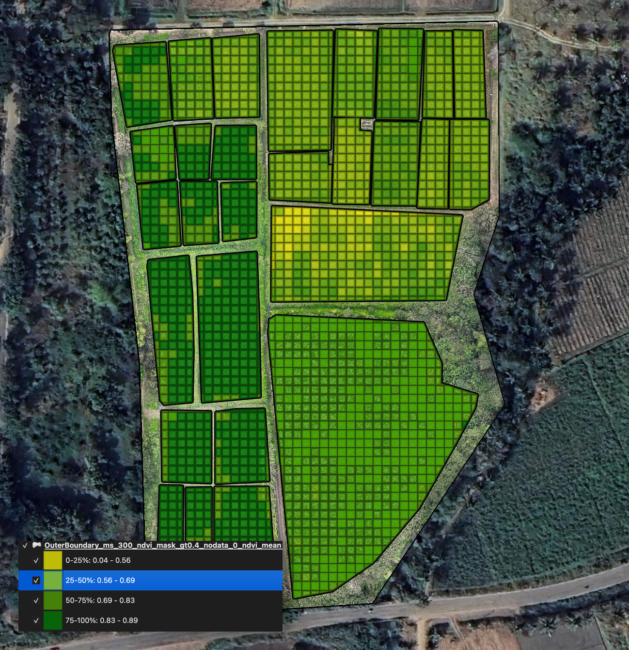
The grid is also the standard input for per-cell raster analysis. Run zonal_statistics.py on grid_clipped.geojson against an NDVI raster to get a mean value per cell, like this:
Get the script
grid_generation.py is part of the Drone Mapping, Terrain & Multispectral Analysis QGIS Package — all 16 QGIS automation scripts at $99 USD.